
In the entire flow of building a machine learning model, you’re now at the blue-highlighted point.

Contents
· Introduction: Why Do We Need Cross Entropy Loss?
· What Happens When We Have More Than Two Options?
· A Practical Example: Let’s Do the Math
∘ Example 1: Binary Cross Entropy
∘ Example 2: Multiclass Cross Entropy
· Conclusion: Why the CE Loss is Such a Big Deal
Suggested Readings
Complete Guide to Training in Machine Learning
Imagine this: you’re building a machine learning model to predict whether an email is spam or not. The model makes its predictions, but here’s the real question: How does it know when it’s messing up?
The solution is the loss function-the model’s personal critic. It tells the model just how wrong it is and by how much. But not all mistakes are created equal. If your model is confidently wrong, the loss function should say: “Wow, you really blew it!”
Cross Entropy Loss is great at this because it penalizes confident mistakes more.
This is why Cross Entropy Loss is so widely used in classification tasks. Whether it’s something simple like predicting spam (binary) or something trickier like figuring out if an image contains a cat, dog, or bird (multiclass), Cross Entropy Loss helps the model learn by making sure it feels the sting of its worst mistakes.
Now that we know why we need it, let’s start with the binary version -because who doesn’t like keeping things simple at first?
Binary Cross Entropy: How Do We Handle Yes or No Questions?
Say you’re building a model to predict whether an email is spam (yes) or not spam (no). How do we measure how bad its predictions are? This is where Binary Cross Entropy comes in.
The formula may look a bit scary at first:

But don’t worry, let’s break it down.
- y_i is the actual label (spam or not spam, 0 or 1).
- p_i is the model’s predicted probability (somewhere between 0 and 1).
Forget about the summation for a moment and just focus on the terms inside the brackets. There are two terms: y_i * log(p_i) and(1 - y_i) * log(1 - p_i) that activate depending on the actual class label y_i.
- If the actual label is 1 (spam), only the first part y_i * log(p_i) is different from 0. If the prediction is close to 1, the loss will be small. If it’s far off (like 0.1), the loss will hit hard, producing a highly negative value.
- If the label is 0 (not spam), we use the second part: (1 - y_i) * log(1 - p_i). If the model predicts 0.8 (very wrong), it’ll feel the pain here.
We repeat this for all n data points and sum the results to get the total loss.
Since logarithms make the total sum negative (because log(x) <= 0 when x <= 1), we add a minus (-) before the summation to get a positive value. To make the loss more interpretable as an average for each sample, we divide by the number of samples n.
Summarizing
In short, Binary Cross Entropy measures how far off the model’s predictions are. If all the predictions are correct than for each data point we will have log(1) = 0 and the total loss will be 0. Conversely if all the predictions are wrong we have log(0) = -∞ for each point and the total loss will be + ∞ thanks to the - in front.
The CE is especially tough on confident mistakes, which is exactly what we want.
Now that we’ve tackled binary classification, the next question is: What happens when we have more than two options? Let’s explore that next.
What Happens When We Have More Than Two Options?
What if your model needs to pick between more than two options? For example, say it’s classifying whether an image shows a cat, a dog, or a bird. How do we measure how wrong the model is when there are multiple classes?
This is where the full version of Cross Entropy Loss comes in, designed for multiclass classification. The principle is the same as in the binary case, but now we’re dealing with multiple predicted probabilities-one for each class.
Here’s the formula, but don’t worry, we’ll break it down:
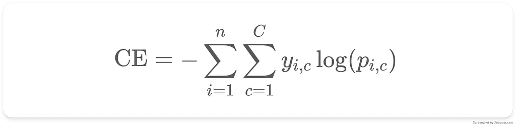
- n is the number of samples.
- C is the number of classes (cat, dog, bird, etc.).
- y_{i,c} is 1 if sample i belongs to class c and 0 otherwise.
- p_{i,c} is the predicted probability that sample i belongs to class c.
What’s Going On Here?
For each sample, the formula focuses only on the correct class, just like in the binary case. This is achieved by the value of y_{i,c} which is 1 only for the class c, the sample i actually belongs to. For the other classes (dog and bird), y_{i,c} would be 0, so the corresponding terms in the formula wouldn’t contribute to the total loss.
Mathematically this is also known as One-Hot Vector, an array that for each datapoint has as many entries as the number of classes, all with value 0 except for the actual class of the datapoint i.
Let’s say the model is 80% sure the image is a cat, 15% sure it’s a dog, and 5% sure it’s a bird:
- If the image is actually a cat, we look only at the log(0.8) term, which gives us a relatively small loss.
- If the model had predicted something crazy, like 0.1 for the cat, the loss would be much larger.
Why Do We Care about Cross Entropy?
The beauty of this loss function is that it penalizes overconfidence in the wrong classes. If the model is 99% sure the image is a bird but it’s actually a cat, the loss will be huge, pushing the model to correct itself.
So, in short, Multiclass Cross Entropy Loss is just an extension of the binary version, but instead of comparing one predicted probability, it compares the model’s confidence across multiple classes.
Now, with both versions in hand, we’ve got the tools to guide our models in making better predictions, whether they’re classifying spam emails or identifying animals in pictures.
A Practical Example: Let’s Do the Math
Let’s bring everything we’ve learned to life with a practical example. We’ll go through both binary and multiclass scenarios to show how Cross Entropy Loss actually calculates the penalty.
Example 1: Binary Cross Entropy
Imagine you have a model predicting whether an email is spam (1) or not spam (0). For a particular email, the actual label is 1 (spam), but the model predicts a 0.3 probability of it being spam.
The formula for Binary Cross Entropy is:

Plugging in our values:
- y_i = 1 (actual label)
- p_i = 0.3 (predicted probability)
Using a calculator, log(0.3) is about -0.52, so:

What does this mean? Since the model was not confident that this email is spam (only 30% sure), the loss is 0.52, indicating a significant penalty. The further the prediction is from 1, the higher this loss would be.
Example 2: Multiclass Cross Entropy
Now let’s take a more complex scenario. Say you have a model predicting whether an image is of a cat, dog, or bird. For one particular image, the actual label is “dog,” but the model predicts the following probabilities:
- Cat: 0.2
- Dog: 0.5
- Bird: 0.3
The formula for Multiclass Cross Entropy is:

For this example, there are three classes (C = 3), and the actual label is dog (y_{i,dog} = 1). Plugging in our values:
Since the log(0.5) is about -0.30, we get:

What does this mean? The model was 50% confident that the image is of a dog, which is correct but not highly confident. The loss is 0.30, indicating some penalty, but less than if the model had given a lower probability for “dog.”

What Did We Learn?
In both examples, Cross Entropy Loss penalizes the model based on how confident it is in its predictions. The more wrong the prediction, and the more confident the model is in that wrong prediction, the higher the loss.
This example shows how Cross Entropy Loss guides the model to adjust its predictions and become more accurate over time-whether it’s deciding between spam and not spam or choosing between a cat, dog, or bird.
Conclusion: Why the CE Loss is Such a Big Deal
The key is in how it penalizes the model’s mistakes. Cross Entropy Loss doesn’t just care if a model is wrong-it cares how wrong and how confident the model was when it made the mistake.
Think of it like a game show. If a contestant says, “I’m 99% sure the answer is ‘cat’,” but the correct answer is “dog,” they’ll lose more points than if they’d said, “I’m not so sure, maybe it’s a cat?” Cross Entropy Loss works the same way: the more confident the wrong answer, the bigger the penalty. This forces the model to improve quickly and adjust its predictions in the right direction.
Seeing the Bigger Picture
Cross Entropy Loss is a favorite in machine learning because it helps models get better, representing a auto-learning tool. It’s like a strict teacher-harsh on mistakes, especially when you should have known better, but effective in guiding you to improve.
Whether the model is working on spam detection (binary) or figuring out whether that blurry shape is a cat, dog, or bird (multiclass), Cross Entropy Loss keeps it honest. It ensures that the model learns from its mistakes and gets better at distinguishing between classes over time.
So, now that we’ve explored the math and the reasoning behind it, you’re equipped with a solid understanding of how Cross Entropy Loss works and why it’s so effective. The next time you see a deep learning model in action, you’ll know how it’s learning from its errors-one penalty at a time.


