Complete Guide to Training in Machine Learning

In the entire flow of building a machine learning model, you’re now at the blue-highlighted point.

Created by the Author

Table of contents:

· Introduction
· Parameter Initialization
· Loss Functions
∘ Purpose
∘ Practical Example: Binary Cross Entropy
∘ Types of Loss Functions
∘ Constructing Loss Functions Using Likelihood
∘ Regularization
· Optimization Algorithms
∘ Purpose
∘ Iterative Algorithms: The Underlying Idea
∘ Types of Optimization Algorithms
∘ Limitations

Suggested Readings

Understanding what a machine learning model is and having a general idea of the training process will give you a nice boost in grasping this article. If you need a refresher, check out the article linked below:

• Supervised Machine Learning: A Simple Explanation for Everyone
• How to Choose the Best Dataset

In this guide, we’ll dive into the three fundamental elements of training a supervised machine learning model on a conceptual level:

Inizializzazione dei parametri

• Parameter Initialization
• Loss functions
• Optmization Algorithms

Parameter Initialization

Just like a good personal trainer, proper parameter initialization ensures your model starts its training with the right foundation, ready to build strength and flexibility in handling data.

The optimization process, which we’ll discuss later, is based on comparing the model’s predicted value with the actual value for each data sample. To make predictions, the model needs to assign initial values to its parameters (represented by ‘β’ in the Binary Logistic Regression formula below).

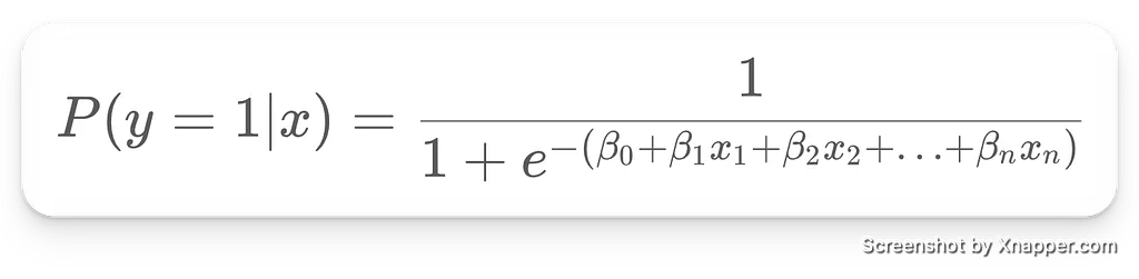
This step, called parameter initialization, is crucial because it sets the model’s starting point before the learning process begins. A good initialization can make the difference between the model finding the lowest cost function value efficiently or getting stuck in a bad spot.

In traditional machine learning, where cost functions are often convex, and algorithms relatively simple, random initialization works just fine. However, in the case of deep learning, random initialization might not cut it due to the complexity of neural networks. That’s where more sophisticated techniques like Xavier and He initialization come into play, but we won’t dive into those here.

Loss Functions

Think of the loss function as your model’s fitness trainer, pushing it to “lose weight” until it’s in the best possible shape to tackle the data’s challenges.

Loss functions usually assume that data is independent and identically distributed (IID), meaning each observation in the dataset comes from the same probability distribution and is independent of the others. While this assumption simplifies analysis and model building, it also introduces some errors.

Although this topic is a bit more technical and won’t be covered in depth here, it’s important to be aware of it.

Purpose

Once the parameters are initialized, the model is ready to make predictions on the data. However, we need a way for the model to evaluate the quality of its predictions and understand how far they deviate from expected values. That’s where the loss function comes in.

Practical Example: Binary Cross Entropy

Let’s look at how a loss function works using one of the most common examples: Binary Cross Entropy, used for binary classification problems where the variables yi e y^i each take on only two values, 0 or 1.

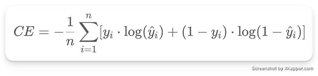
Where:

• $n$ is the number of observations in the dataset.
• $y_i$ is the actual value of observation ‘i’, either 0 or 1.
• $\hat{y}_i$ is the predicted value for observation ‘i’, also either 0 or 1.

Forget the summation and just focus on the part inside the square brackets. There are two terms, $y_i \log(\hat{y}_i)$ and $(1 - y_i) \log(1 - \hat{y}_i)$:

• $y_i \log(\hat{y}_i)$: this equals 0 when the true class is 0, and it equals $\log(\hat{y}_i)$ when the true class is 1.
• $(1 - y_i) \log(1 - \hat{y}_i)$: equals 0 when the class is 1 and has a value if $y_i = 0$.

We can split the loss function into two parts: CEpos ($y_i = 1$) and CEneg ($y_i = 0$).

Part 1: Positive Class Samples

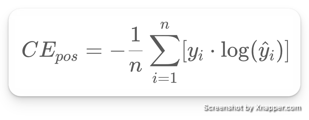
This represents the loss for all class 1 points. Take point ‘i’ and calculate its loss by applying the logarithm to the model’s predicted value for that point. If the predicted value is 1, the impact on the loss will be zero log(1) = 0, but if it’s different, say 0.3, the loss will be log(0.3). This process is repeated for all points in the training set, and the resulting losses are summed.

Part 2: Negative Class Samples

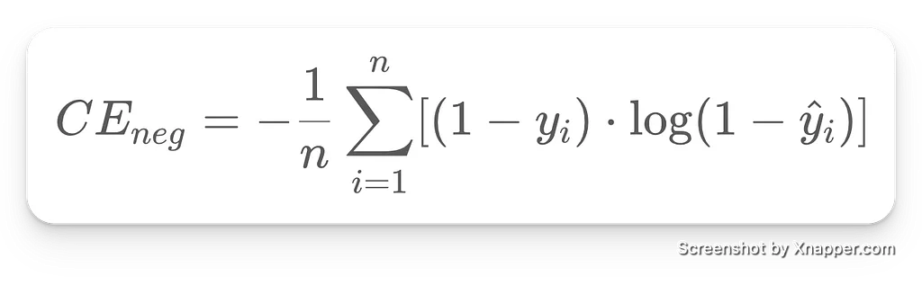
The same thing happens here, but for each negative sample. If the predicted value is 0, the impact on the loss will be log(1 - 0) = 0, so no harm done. If not, we’ll get a different value.

Total CE

At the end of the day, CE assigns a loss value to every sample the model misclassifies. The sum of these values is our total loss, which optimization algorithms will work on.

Nota: Want a numerical example or deeper mathematical explanation of cross entropy? Click here.

Types of Loss Functions

Different machine learning problems, such as classification and regression, require different approaches to evaluate model performance. Therefore, various types of loss functions are used, designed to fit the specific needs of each type of problem.

In this section, we simply list some of the most common loss functions for awareness. A deeper analysis will come in due time, with dedicated articles available in section 5 of the model creation flow.

Loss Functions for Regression

• MSE (Mean Squared Error)
• MAE (Mean Absolute Error)
• MAPE (Mean Absolute Percentage Error)

Loss Functions for Classification

• Cross-Entropy Loss (Binary)
• Cross-Entropy Loss (Multiclass)
• Hinge Loss (SVM)

Constructing Loss Functions Using Likelihood

ll these loss functions look great, but who invented them? Why are they made this way? If you’ve ever asked yourself these questions, here’s the answer: likelihood.

Most loss functions are built with the goal of maximizing the probability that our model, given its parameter values, returns data as close as possible to the training data. This is expressed in the following formula.

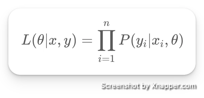
This part is a bit more technical and goes beyond the scope of this article, but you’ll find a dedicated post in our stories.

Regularization

Regularization is a key concept in model training, used to prevent overfitting and improve a model’s generalization. It’s often integrated directly into the loss functions by adding regularization terms.

The idea is quite simple: we add a value to our loss that depends on the parameters. In the case of binary cross-entropy with L2 regularization (illustrated below), it looks like this:

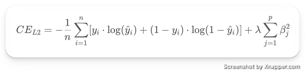
This way, when our model has many parameters with high values, it suffers a greater loss. This encourages the model to find a balance between classification accuracy and model complexity by reducing the magnitude of the parameters.

During training, the parameters are adjusted to minimize the overall penalty, focusing particularly on reducing those parameters that contribute less to the model’s accuracy. In practice, if an influential parameter is reduced, the associated classification loss increases, pushing the model to keep that parameter intact. Conversely, less important parameters can be reduced with fewer consequences on the overall loss, promoting a simpler model.

At the end of the training process, we achieve an optimal balance between model complexity and its ability to generalize. This means finding the right compromise between a complex, flexible model that risks overfitting the training data, and a too-simple model that might not capture enough information from the data.

Ridge Regression (L2):

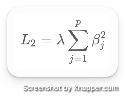
• Description: Adds a regularization term based on the square of the parameters to the loss function. It strongly reduces certain parameter values and lowers the model’s complexity to prevent overfitting.

Lasso Regression (L1):

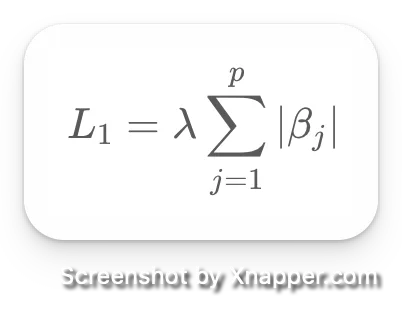
• Description: Adds a regularization term based on the absolute value of the parameters to the loss function. It can completely eliminate certain parameters, resulting in sparse models.

Optimization Algorithms

If the loss function is your model’s personal trainer, optimization algorithms are like a range of gym equipment. Each one offers a different way to shape and sculpt your model’s weights (parameters).

Purpose

We’ve seen that the loss function measures the error made by the model. Now, we need something that can figure out how to reduce that error. In other words, we need an algorithm that tells the model how to adjust the parameters to minimize the loss.

There are two main ways to optimize: one is more direct, solving equations, which is useful for simple problems like linear regression. In this case, the optimal value of the parameters is the solution of the equation or system of equations.

However, in many cases, equations alone won’t cut it, so we turn to iterative approaches. In this approach, the parameter values are approximated with each iteration, progressively getting closer to the solution. The optimal solution isn’t always reached, but we aim to get as close as possible. These are the most common algorithms in machine learning, which this section focuses on.

Iterative Algorithms: The Underlying Idea

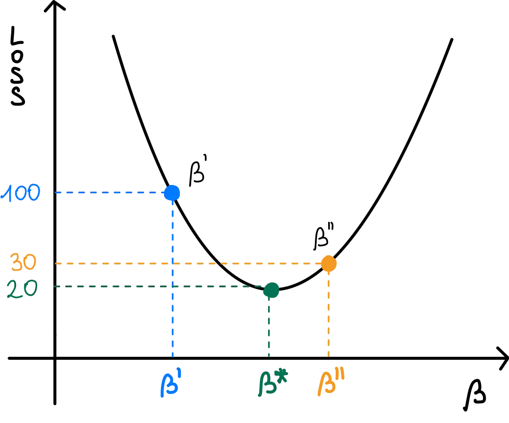
Iterative optimization algorithms work in steps, based on gradient calculation. At each step, they assess the slope of the loss function at a specific point and move in the opposite direction to reduce the error. This cycle repeats until a termination criterion is met. Typically, this happens when the difference between the loss values of two consecutive iterations is smaller than a predefined threshold, or when a maximum number of iterations is reached.

At the end of the process, the parameters will have values that allow the model to make better predictions, as they approach the loss function’s minimum point.

Drawn by the Author

This mechanism works perfectly when we’re dealing with convex functions like the one shown in the figure.

If our parameters are at the blue point, the slope (derivative) is calculated at (β’, 100), and in this case, it would be negative. Therefore, the parameters will be increased, moving in the direction of the minimum point. If, with this increase, the new parameters are at the orange point, then the derivative at (β”, 30) will be positive, so the parameters will be reduced, moving left again towards the minimum point, which is exactly reached in this case.

Types of Optimization Algorithms

Formula Legend:

θ represents the model’s parameters

α is the learning rate

J(θ) is the loss function

∇J(θ) is the gradient of the loss function with respect to the parameters

B is a mini-batch of data

$x_i$ is a single point from the training set

Gradient Descent (GD):

GD is an iterative process that, at each step, calculates the loss for every point in the training dataset, computes the derivative of the loss, and updates the parameters in the opposite direction. The parameter update formula is:

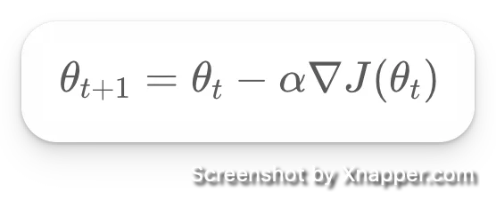
GD produces a steady, gradual decrease in the loss because the direction taken is accurate, as it’s based on the entire training set. However, this also leads to significant computational complexity.

Mini Batch Gradient Descent (MBGD):

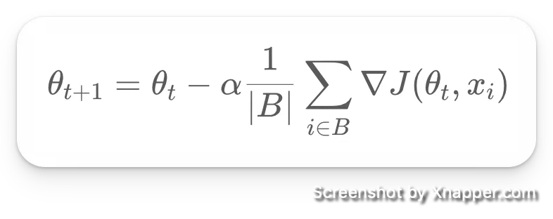
MBGD is similar to GD, but only considers a subset (batch) of the training points at each iteration. This results in greater computational efficiency but might make the loss slightly less stable. The choice of batch size is crucial.

Stochastic Gradient Descent (SGD):

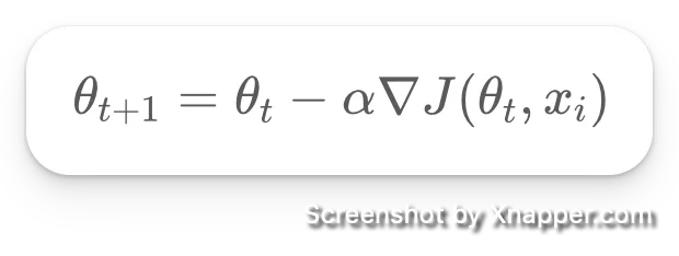
SGD takes the reduction to the extreme by considering just one point at a time in each iteration. This approach makes the loss more unstable, as basing updates on a single point might not always be correct. However, when executed over enough iterations, the overall direction of the updates will, on average, be correct. This gives SGD tremendous computational efficiency.

Limitations

These algorithms may struggle when the loss function is non-convex, which is common in deep learning problems. To tackle this, special techniques like momentum (not covered here) have been introduced. Moreover, in deep learning, more advanced techniques like Adam have been developed to handle the high complexity of neural architectures.